Abstract
The task of classifying the accent of recorded speech has generally been approached with traditional SVM or UBM-GMM methods (Omar and Pelecanos, 2010; Ge, 2015). However, modern deep learning methods yield the potential to dramatically increase performance. In our report, we train several varieties of Recurrent and Convolutional Neural Networks on three types of features (MFCC, formant, and raw spectrogram) extracted from North American and British English speech recordings in order to predict the accent of the speaker. All deep learning methods examined surpass non-deep baselines, and the approach yielding the best performance was the MFCC-RNN, shortly followed by the Spec-CNN.
Background
Treating speech audio using automatic techniques has long been a staple of the machine learning field. These techniques culminate in the construction of Automatic Speech Recognition (ASR) systems, which have a wide variety of applications including speech-to-text utilities, electronic personal assistants, and automatic translation systems. While ability to recognize speech automatically has increased dramatically over the past decade due to the advent of deep neural networks, ASR systems still are at the mercy of their input data: human speech is highly variable, influenced by recording noise and by the age, sex, accent, and other characteristics of the speaker.
In particular, two individuals speaking the same sentence in the same language might receive different results from the ASR pipeline if they have two different regional accents. A simple solution might be to train two ASR models, one per expected accent, and to perform accent classification on input audio to determine which model to use for downstream tasks. To this end, we explore several predictive models from a variety of machine learning algorithms to classify English speech audio according to the accent of the speaker. Traditionally, accent classification has been approached with SVM or UBM-GMM methods (Omar and Pelecanos, 2010; Ge, 2015), but we are motivated to take advantage of recent deep learning techniques to potentially improve upon this performance.
Convolutional Neural Networks (CNNs) have been shown to be useful for audio classification tasks. Hershey et al. (2016) explored the performance of several CNN based models, including a fully- connected CNN model and several preexisting architectures such as VGG, Inception, and Resnet, on the classification of 70 million YouTube videos, each tagged with a content label such as sports or singing, using log-mel spectrograms to represent the audio features of the videos. They achieve an AUC of 92.6% using Resnet-50 and 85.1% using their fully-connected model. Chen, Shen, and Tang (2018) performed a binary classification task (native vs. non-native) using the CMU ARCTIC corpus, which contains recordings of US English and other varieties of accented English. They trained a CNN model with 10 convolutional layers and one fully-connected layer on log-amplitude spectrograms representing speech audio segments, reaching a classification accuracy of 97.8%.
Flavours of Recurrent Neural Networks (RNNs) have also been used for the task of accent classifica- tion. Chu, Lai, and Le (2017) used a Long Short-Term Memory (LSTM) network to classify speech audio segments represented by its Mel-frequency cepstral coefficients (MFCCs) and delta features into 5 accents, yielding only a 39.8% classification accuracy. Since their accuracy on the test set was getting better with more training inputs, the authors did mention that a bigger dataset would improve their performance.
In this work, we perform a comparative study of techniques used in accent classification, varying both feature extraction methods and learning algorithms. We aim to classify recordings of English speech into British vs. North American accents, comparing the performance of an RNN trained on MFCC features, an RNN trained on formant features, and a CNN trained on raw spectrogram features. Our effort is to find which combination of feature extraction and deep learning approaches yields most accurate classification results.
Methodology
Datasets and preprocessing
The audio for the North-American English comes from the “test” subset of the Librispeech Corpus, which is assembled from clean single-speaker recordings of North American audiobook narrators from the open-source public-domain website Librivox (Panayotov et al., 2015). Since no equivalent- quality British English spoken corpus could be found, we assembled the Librit Corpus, a corpus of recordings of British audiobook narrators also sourced from Librivox. Our versions of Librispeech and Librit contain about 5.5 and 7 hours of audio from 40 and 27 speakers respectively, roughly balanced male and female.
Audio from both corpora was downsampled to 16 kHz mono .wav files, and then split into 20-second clips. While silence is often removed in speech processing tasks, we elected not to do so, because it is possible that natural pauses in speech could be a cue for accent learnable by a classifier.
Feature extraction
We extract three types of features from our audio in order to explore which is most informative for this task. The first are Mel-frequency cepstral coefficients (MFCCs), a standard in speech processing that is loosely modelled on the processing of the human ear. For each frame of the audio, we calculate its power spectrum, take the logarithm of the summed energies after applying the Mel filterbank, and keep the first 13 coefficients from the discrete cosine transform of these log filterbank energies.
The second type of feature we extract are the formant features. Previous research suggests that formants, the vocal tract resonant frequencies measured when a vowel or similar voiced sound is produced, are a salient cue for accent detection (Hansen and Arslan, 1995). Hence, we extract the first three formants from every voiced frame in the audio, following the heuristic of Deshpande, Chikkerur, and Govindaraju (2005): we consider a frame voiced if its log energy is greater than or equal to -9.0, and if its number of zero-crossings is between 1 and 45.
Thirdly, we apply a Fourier transform to the time signal of the audio, generating a spectrogram. We then save the raw spectrogram features, i.e., the frequency, amplitude, and time values needed to visually represent the spectrogram for that audio file.
Proposed networks
Since the MFCC and formant features are inherently sequential, being extracted from a series of time frames, they are suitable for use with a Recurrent Neural Network (RNN). We propose a Long Short-Term Memory Network (LSTM) for each of these features, since these are especially suited for “remembering” information from many steps into the past, which applies well given the large number of frames in our 20-second examples. We call these the MFCC-RNN and the Formant-RNN respectively.
Traditionally, Convolutional Neural Networks (CNNs) are used for computer vision tasks to recognize colours, edges, and contours of objects. We follow others in applying this approach to audio data, where the CNN treats the spectrogram representation roughly as an image that contains “objects” reflective of speech characteristics (Chen, Shen, and Tang, 2018; Hershey et al., 2016). Rather than pre-selecting features using speech-specific processing derived by linguists, the CNN learns 2 low-level audio features present in the raw spectrogram, potentially capturing speech characteristics not quantified by MFCCs or formant measurements. We call this network the Spec-CNN.
Experiments
We split our data into 90% training and 10% testing, or 80% training, 10% validation, 10% testing where appropriate. For each feature, in addition to the relevant trained network, we also test a Most Frequent (MF) baseline that always chooses the class label most frequent in the training data (since our examples do not contain the exact same amount of data from each class, and sometimes variations in preprocessing cause slight differences in the amount of data for which features can be extracted), and an (rbf) SVM baseline. In order to be considered useful, the network must outperform the MF baseline, and it is desirable that it also outperform the SVM baseline. For details on the hyperparameter tuning for all networks, and for detailed diagrams on network architectures, see Appendices B and C.
For the MF and SVM baselines, “flattened” versions of the MFCC and formant features were used, which collapsed the features across the time dimension, since these classifiers do not take sequential data as input.
MFCC features (MFCC-RNN)
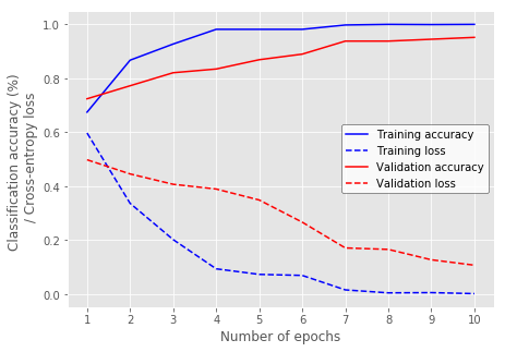
For the MFCC-RNN, we train an LSTM with one hidden layer and 350 hidden units using an Adam optimizer and cross-entropy loss over 10 epochs. The classification accuracies and the learning curves of the MFCC-RNN can be found in Table 1 and Figure 1 respectively.
| Classifier | Train | Valid | Test |
|---|---|---|---|
| (%) | (%) | (%) | |
| MF | 63.33 | - | 59.23 |
| SVM | 100.00 | - | 61.71 |
| MFCC-RNN | 100.00 | 95.17 | 95.32 |
Formant features (Formant-RNN)
For the Formant-RNN, we train a bidirectional LSTM with one hidden layer of 200 hidden units, three dense layers with 1024 hidden units, and a fourth dense layer with 2048 hidden units. Dropout with probability of 0.3 was added to all of the previous dense layers. The network was trained over 26 epochs (early stopped) using an Adam optimizer and a cross-entropy loss. The classification accuracies and the learning curves of the Formant-RNN can be found in Table 2 and Figure 2 respectively.
| Classifier | Train | Valid | Test |
|---|---|---|---|
| (%) | (%) | (%) | |
| MF | 53.35 | - | 55.07 |
| SVM | 100.00 | - | 55.07 |
| Formant-RNN | 99.06 | 90.96 | 86.96 |
Raw spectrogram features (Spec-CNN)
As outlined in Section 2.1, input data initially consisted of 20 second audio clips, but the spectrogram generated was too large for efficient training of CNNs. Thus, following the practice of Hershey et al. (2016) who also trained on spectrogram data, we further sliced our audio into one-second clips, yielding 19475 North American accent examples and 22541 British accent examples. We then generated spectrograms every 10 ms, using a 25 ms window which gives sufficient time and frequency resolution to resolve features in the spectrogram. The spectrograms thus generated have dimensions of 201 frequency bins between 0-8000 Hz and 66 bins along the one-second time axis.
| Classifier | Train | Valid | Test |
|---|---|---|---|
| (%) | (%) | (%) | |
| MF | 54.52 | - | 53.67 |
| SVM | 99.98 | - | 53.67 |
| Spec-CNN | 98.12 | 94.57 | 92.63 |
Discussion
All three of our deep-learning classifiers (MFCC-RNN, Formant-RNN, and Spec-CNN) are able to outperform both the MF and SVM baselines. The classifier performing the best was the MFCC-RNN, yielding a test accuracy of 95.32%. This combination of feature and learning algorithm seems to strike the right balance for the characterization of speech: MFCCs make use of a large amount of frequency information, and the RNN approach allows previous contextual information to be modelled, which helps account for many progressive phonetic processes that are probably cues for accent. The MFCC features also use information from the entire signal, and not just from heuristically-chosen speech segments, permitting more nuanced modelling.
The Spec-CNN earns a close second with test accuracy 92.63%. The raw spectrogram features contain nearly three times more information than the MFCC- or Formant-RNNs, comprising frequency and amplitude information for each frame; this large amount of information is likely responsible for much of the classification accuracy. However, since splitting the audio further into one-second clips was necessary, contextual information that the other networks have is lost to Spec-CNN. Moreover, the large size of the spectrogram information, which likely includes significant amounts of noise, means that a more complex model is needed to learn the important features within it, and thus a larger amount of data is needed to yield significant improvement in accuracy. We speculate that larger training corpora might give higher performance, and that timescales longer than one second might also boost accuracy due to a higher number of contextual clues.
The Formant-RNN, while far sparser in terms of frequency information than the MFCC-RNN, still performs relatively well with 86.96% test accuracy. Its ability to still recover most of the accent cues that the MFCC-RNN detects is likely bolstered by the bidirectional nature of the RNN, which may help model the regressive as well as the progressive phonetic processes present in the audio. However, since formant features are only extracted from heuristically-chosen voiced frames, this classifier is limited not only by the accuracy of the heuristic but also by the number of accent cues present in only the voiced frames. For example, many North American speakers pronounce schedule with a [k], while British speakers use [S], but since neither of these sounds are voiced, this cue cannot be learned by the Formant-RNN.
There is a practical tradeoff regarding dataset size, computational time, and accuracy: while the Spec-CNN is potentially capable of leveraging a detailed signal into high accuracy, it requires lots of data and computational power (including navigation of GPU and RAM limits). The MFCC-RNN offers similar performance in less time, and is thus suited for smaller datasets. The Formant-RNN, while the easiest to train of the three, yields the lowest performance due to the under-salient cues it learns.
Learned features
As expected, the networks do learn to “pay attention” to different features. This is visualized in Figure 4, which shows the influence of each subsection of audio on the final classification outcome for one training example. In the RNN cases, we perturb the time steps one at a time by a small value and calculate the difference in classification probabilities between the original sequence and the sequence with the perturbed time step. The larger the difference between these probabilities, the more influential we consider the time step (represented by a yellower colour). In the CNN case, we use the keras-vis API to visualize the learned weights of the convolution filters, where higher weights yield brighter colours and correspond to more important features.
Qualitative examination of the (British) audio1alongside Figure 4a suggests that the MFCC-RNN sometimes learns something somewhat compatible with human intuition. From left to right, the red boxes roughly correspond to instances of the vowels [6], [O], and [œ] (the sounds in Feuerbach, *org, and another rendering of *Feuerbach\), respectively, which are vowels more common to British dialects than American ones. There are many other yellow bands such as these, suggesting that the MFCC-RNN also learns less transparently interpretable features (i.e., without a perfect correspondence to a human notion such as a particular vowel) used as accent cues.
In Figure 4b, we observe a much starker difference between more- and less-influential segments (bluer and yellower, respectively). This is due to the lower dimensionality of the input features. In red are boxed the same vowel instances as are found by the MFCC-RNN, and on the whole there seems to be some degree of correspondence between what these two RNNs learn. This is perhaps surprising, since the MFCC data is much more complex and incorporates much more of the signal information than the formant data, which is simply three frequency measurements per voiced frame.
Figure 4c shows what is treated as important by the final layer of the Spec-CNN. The network pays attention to different features at different convolutional layers (with layer-by-layer diagrams available in Appendix D). In the second convolutional layer, the Spec-CNN weights still resemble a spectrum and it focuses on the lower frequencies, where most salient speech information is aggregated. However, as we go to the third convolutional layer, the weights are abstracted from the notion of a frequency spectrum, spanning more space in the y direction. Research in deep learning is still being done on interpretability of the learned representations; for this reason, we choose not to label y-axis of the CNN (Olah et al., 2018). The red-boxed intervals on the x-axis in Figure 4c highlighted by Spec-CNN correspond to where the speaker pronounces iconically British vowels, as observed in the RNNs. Therefore, we empirically conjecture that Spec-CNN abstracts away the frequency axis per se and pays attention to the important time intervals. We remark that our two general methods (RNN and CNN) roughly “agree” with each other regarding which segments are important.
Conclusion and future work
The MFCC-RNN performs best on our accent classification task, likely due to its sufficiently complex and salient features and its ability to take contextual information into account, and its performance is shortly followed by that of the the Spec-CNN (which may outperform the MFCC-RNN given more data and more computational power). The Formant-RNN performs worst of the three, likely due to the excessively low amount of information present in its features.
A straightforward next step in evaluating these network architectures and feature choices would be to extend them beyond binary classification, including data from many varieties of English. This would allow a more direct comparison with works such as Chu, Lai, and Le (2017), which was unable to classify multiple varieties of accented English well using an MFCC approach.
Further future work might include expansion on the Spec-CNN, since current research continues to look into new types of convolution to curate filters for audio signals. One successful application of CNNs with raw audio involves using parametrized sinc functions in the convolution layer instead of a traditional convolution, as in SincNet developed by Ravanelli and Bengio (2018). Dilated convolutions have also been shown to be useful for accent correction and audio generation, since they allow the receptive fields to grow longer in a cheaper way than do LSTMs or other RNNs (Oord et al., 2016).
Though it underperformed in this work, the above-baseline performance of the Formant-RNN also holds potential due to the easy interpretability of its features. Future work might construct a mapping from the features picked out as important by the network back to their original timestamp, which could be the basis of an accent correction system that delivers feedback to a user about which portions of their speech need adjustment in order to imitate a certain accent. This is especially applicable to the Formant-RNN since there is a well-understood relationship between the configuration of the mouth and the first two formants of a vowel. Such a system could provide practical instructions to the user (i.e. to raise or lower the tongue, round the lips, etc.) and could have applications in language learning or speech therapy tools.
Appendix
A sample dataset
In the project repo, we include 1020sec.wav, a 20 second file from Librit (our British audio corpus). In our report, we specify that our neural networks identify the following:
| Phoneme | Word of the phoneme | Time Window in Audio (seconds) |
|---|---|---|
| eu | Feuerbach | 1:49 to 2:19 |
| or | org | 10:86 to 11:39 |
| eu | Feuerbach | 17:65 to 18:41 |
You can play the audio using any open source or commercial audio player to skip to the following timestamps and verify our results. Additionally, the image files showing the visualization of the weights learned by the neural network are available here in higher resolution.
B Hyperparameter tuning on validation set
Hyperparameter values for the RNNs were tuned in a heuristic manner, as we lack the computational resources to systematically check each possible combination. For the CNN, a grid search method was used. For all cases, we choose the hyperparameter values that give the highest classification accuracy on the validation set. This ensures we are not overfitting to the training data.
B.1 MFCC-RNN
| Number of epochs | Number of hidden units | Train | Valid | Test |
|---|---|---|---|---|
| 10 | 100 | 99.92 | 83.45 | 80.17 |
| 10 | 200 | 99.85 | 90.10 | 92.01 |
| 10 | 300 | 99.46 | 87.57 | 92.56 |
| 6 | 325 | 98.54 | 88.97 | 88.71 |
| 10 | 350 | 100.00 | 95.17 | 95.32 |
| 10 | 375 | 96.16 | 93.10 | 96.14 |
| 6 | 400 | 99.23 | 88.28 | 90.63 |
Table 5: Percent classification accuracies using various hyperparameter values on the MFCC-RNN
B.2 Formant-RNN
| Number of hidden units | Valid |
|---|---|
| 10 | 0.58 |
| 20 | 0.56 |
| 50 | 0.62 |
| 100 | 0.63 |
| 200 | 0.74 |
Table 6: accuracy using various numbers of hidden units on the Formant-RNN (tuned over 20 epochs)
B.3 Spec-CNN
| Acitvation function | Valid |
|---|---|
| Softmax | 0.630513 |
| Softplus | 0.791683 |
| Softsign | 0.879486 |
| Relu | 0.815786 |
| Tanh | 0.895775 |
| Sigmoid | 0.699378 |
| Hard_sigmoid | 0.693815 |
| Linear | 0.705999 |
| learning rate | Valid |
|---|---|
| 0.00001 | 0.551715 |
| 0.0001 | 0.686002 |
| 0.001 | 0.823864 |
| 0.01 | 0.544828 |
| 0.1 | 0.481128 |
| Convolution kernel size | valid |
|---|---|
| 3 | 0.815786 |
| 4 | 0.796318 |
| 5 | 0.003469 |
| Initialization mode for kernel | Valid |
|---|---|
| uniform | 0.888756 |
| lecun_uniform | 0.872997 |
| normal | 0.890081 |
| zero | 0.545226 |
| glorot_normal | 0.890081 |
| glorot_uniform | 0.883989 |
| he_normal | 0.831148 |
| he_uniform | 0.843729 |
| Optimizer | Valid |
|---|---|
| SGD | 0.679115 |
| RMSprop | 0.818037 |
| Adagrad | 0.624421 |
| Adadelta | 0.527480 |
| Adam | 0.808767 |
| Adamax | 0.723348 |
| Nadam | 0.790094 |
Authors (alphabetical order)
- Jonathan Bhimani-Burrows
- Khalil Bibi
- Arlie Coles
- Akila Jeeson Daniel
- Violet Guo
- Louis-François Préville-Ratelle
Citations and figures are available upon request.